- नवाचार
- PCI के आवेदन पर लेख
- पोर्टफोलियो ट्रेडिंग
Portfolio Quoting Method for Analysis of "Good" and "Bad" Portfolios
The global financial crisis of 2008 affected all sectors of economic activity with no exception. It affected the business performance of companies both directly and indirectly, but the level of impact was different. This fact provides broad opportunities to find investment strategies based on differences in the long-term price reaction of, for instance, stocks on the same systematic factor.
In this article we will try to find an example of a portfolio that would statistically and graphically reflect the possibility of building a successful investment strategy based on differences in the long-term behavior of stocks. For this purpose, we selected 22 stocks of U.S. large and liquid companies belonging to the various sectors of the economy. Using the approaches of modern portfolio theory, the principles of risk diversification, as well as the method of portfolio quoting PQM, we will try to divide our selected assets into 2 groups: "Good" portfolio and "Bad" portfolio.
The “Good” portfolio will consist of assets with positive weights, that is, candidates for purchase. The “Bad” portfolio will include stocks on which short positions should be taken according to our analysis. The entire analysis is based on monthly closing prices recorded over the past 4 years (50 months). The composition of the assets (22 shares), selected to build a portfolio, with corresponding tickers, Company names and economic sectors are given below:
Table 1: Company names and economic sectors of the selected shares
| # | Ticker | Company | Sector |
| 1 | AA | AlcoaInc | BasicMaterials |
| 2 | AXP | AmericanExpressCompany | Financials |
| 3 | BA | BoeingCompany | Industrials |
| 4 | DD | DupontCompany | BasicMaterials |
| 5 | DIS | WaltDisneyCompany | CyclicalConsumerGoods&Services |
| 6 | GE | GeneralElectricCorporation | Industrials |
| 7 | HD | HomeDepotInc | CyclicalConsumerGoods&Services |
| 8 | HON | HoneywellInternationalInc | Industrials |
| 9 | HPQ | Hewlett-PackardCompany | Technology |
| 10 | IBM | InternationalBusinessMachineCorp | Technology |
| 11 | INTC | IntelCorporation | Technology |
| 12 | JNJ | Johnson&Johnson | Healthcare |
| 13 | JPM | JP MorganChase&Company | Financials |
| 14 | KO | Coca-ColaCompany | ConsumerNon-Cyclicals |
| 15 | MCD | McDonaldsCorporation | CyclicalConsumerGoods&Services |
| 16 | MRK | MerckCoInc | Healthcare |
| 17 | MSFT | MicrosoftCorporation | Technology |
| 18 | PFE | PfizerInc | Healthcare |
| 19 | T | AT&T | Telecommunication |
| 20 | VZ | VerizonCommunicationsInc | Telecommunication |
| 21 | WMT | Wal-MartStoresInc | CyclicalConsumerGoods&Services |
| 22 | XOM | ExxonMobilCorporation | Energy |
On the basis of monthly data, let us calculate realized values of the average return, the standard deviation of return, and a simplified version of the Sharpe ratio for each data series.
The results of the calculations of average monthly returns and standard deviations are shown in the table below:
Table 2: Average monthly returns and standard deviations
| Asset | MeanReturn | StandardDeviation | Asset | MeanReturn | StandardDeviation |
| AA | 0.31% | 10.60% | JNJ | 1.01% | 3.76% |
| AXP | 3.32% | 10.96% | JPM | 1.27% | 9.05% |
| BA | 1.99% | 6.96% | KO | 1.31% | 4.16% |
| DD | 1.81% | 7.90% | MCD | 1.22% | 3.68% |
| DIS | 2.58% | 6.54% | MRK | 1.11% | 5.28% |
| GE | 1.64% | 8.48% | MSFT | 1.20% | 6.67% |
| HD | 2.33% | 6.41% | PFE | 1.54% | 4.85% |
| HON | 2.05% | 6.40% | T | 0.78% | 4.16% |
| HPQ | -0.80% | 10.36% | VZ | 1.27% | 4.83% |
| IBM | 1.49% | 4.27% | WMT | 0.83% | 4.17% |
| INTC | 0.92% | 6.59% | XOM | 0.58% | 4.65% |
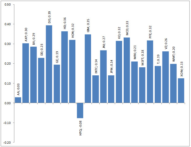
In addition, we can calculate a simplified version of the Sharpe ratio for each asset. The ratio results from dividing the return by the standard deviation and shows the return per unit of risk. These coefficients will be a good guide for our analysis in order to determine the effectiveness of the investment strategy. The resulting coefficients are shown in the diagram:
Diagram 1: Sharpe ratios of the selected shares

The next stage of the analysis is to find optimal weight coefficients for each asset and to build a stock portfolio. The optimality criterion for the portfolio may be the Sharpe ratio, the parameter of return or its standard deviation. In our case, the optimality criterion will be the maximum possible portfolio expected return, achievable at all levels of standard deviation not higher than the average standard deviation for the sample of 22 stocks. The average standard deviation for the 22 stocks is 6.40% and we want our portfolio not to be more risky than its constituent assets on average. To calculate weight coefficients, we will also need the covariance of assets, which indicate the level of interrelationship between each pair of assets.
The weight optimization procedure (having two constraints: the maximum standard deviation of the portfolio (6.40%) and the final sum of the weights, which should be 100%) leads us to the following solution, which maximizes the return of the portfolio:
Table 3: Optimized weights for each asset
| Asset | Weight | Asset | Weight |
| AA | -70.27% | JNJ | 21.59% |
| AXP | 8.97% | JPM | -31.82% |
| BA | -4.39% | KO | 29.55% |
| DD | -22.00% | MCD | -15.80% |
| DIS | 88.08% | MRK | -5.98% |
| GE | -41.55% | MSFT | 51.73% |
| HD | 37.01% | PFE | 39.28% |
| HON | 145.66% | T | -96.14% |
| HPQ | -43.92% | VZ | 81.77% |
| IBM | 152.36% | WMT | -56.03% |
| INTC | -39.34% | XOM | -128.76% |
Since we did not put restrictions on the possibility of short sales of assets, the solution gives both positive and negative weights. The assets with positive weights will conditionally be called "Good" and the ones with negative weight- "Bad" portfolios. Let us regroup the assets in accordance with their new classification:
Table 4: Optimized weights for investment portfolio
| GoodPortfolio | BadPortfolio |
| Asset | Weight | Asset | Weight |
| AXP | 8.97% | AA | -70.27% |
| DIS | 88.08% | BA | -4.39% |
| HD | 37.01% | DD | -22.00% |
| HON | 145.66% | GE | -41.55% |
| IBM | 152.36% | HPQ | -43.92% |
| JNJ | 21.59% | INTC | -39.34% |
| KO | 29.55% | JPM | -31.82% |
| MSFT | 51.73% | MCD | -15.80% |
| PFE | 39.28% | MRK | -5.98% |
| VZ | 81.77% | T | -96.14% |
| WMT | -56.03% | ||
| XOM | -128.76% |
There are slightly more "Bad" assets than the "Good" ones; however, such an epithet does not diminish their importance. As we will see later, these two groups of assets are able to show the most effective performance only when they are together. As for companies’ belonging to an economic sector, we could not highlight a specific pattern for the companies entering a certain portfolio. Companies, representing completely different sectors, were included in both portfolios.
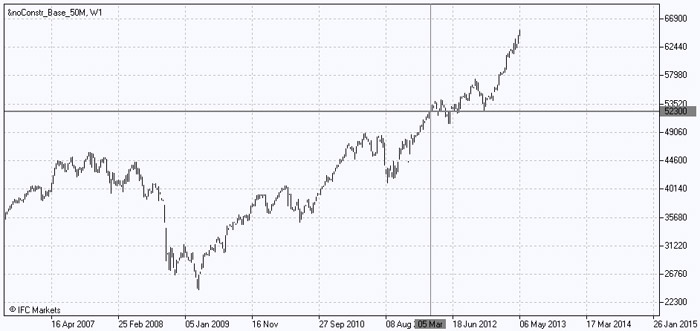
Let us now display "Good" and "Bad" portfolio charts separately. We will use the method of portfolio quotinh PQM, which is implemented in trading-analytical terminal NetTradeX. We choose 10 assets from "Good" portfolio and express its value in U.S. dollars as we are now interested in looking at its absolute value. To do this, we introduce weight coefficient for each asset in terms of U.S. dollars, at the same time respecting the proportion, obtained previously in the solution for the optimal portfolio. For example, for AXP stocks we are entering the amount of 897 dollars and for the stock VZ, the volume of 8177 dollars. Despite that the volume was set in dollars, not in percentage, it will not affect the shape of portfolio’s curve, but only the coordinates. The chart is as follows:
Chart 1: Absolute Value of the Portfolio of Longs

In general, we have a growing retrospective structure. Since the beginning of January 2009 the value of the "Good" portfolio increased by 2.5 times, but we should also mention a significant fall in the portfolio value in 2008. Let us also note that in the beginning of March 2012 the portfolio's value fluctuated around 52,300 dollars; this fact will help us in future for studying the dynamics of the combined portfolio.
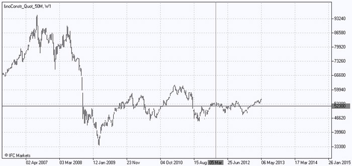
Similarly, we will construct the "Bad" portfolio consisting of 12 assets, introducing the corresponding volumes in U.S. dollars. Its retrospective dynamics is presented on the chart:
Chart 2: Absolute Value of the Portfolio Short

Obviously, the "Bad" portfolio justifies its name, having significantly underperformed the "Good” portfolio in terms of realized return, which is evident from the three-fold decrease in its value in 2008 and the subsequent slight growth. In addition, let us note that at the beginning of March 2012 the value of "Bad" portfolio also fluctuated around 52,300 dollars.
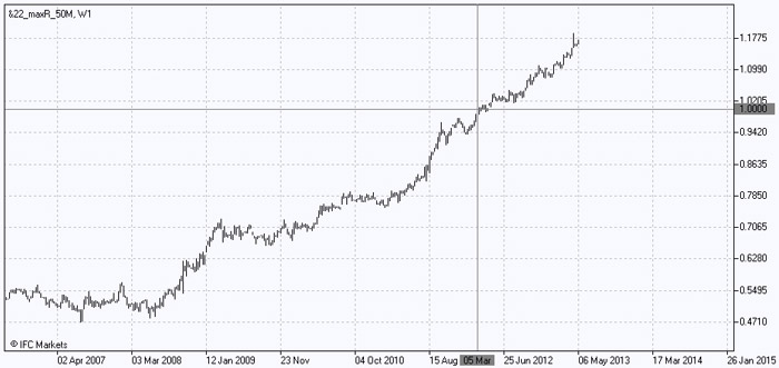
Finally, we will construct a combined portfolio which will include both "Good" and "Bad" assets with those weights obtained during the optimization. Note that the negative weights correspond to short selling of the asset. When building a portfolio in trading and analytical terminal NetTradeX, assets with positive weights will be included in the base part of the composite portfolio, while assets with short weights - in the quoted part. In other words, we conditionally buy assets of "Good" portfolio and sell assets of the "Bad" one – these two actions reflect the essence of PQM method. The result is a coefficient that reflects the value of the first (in our case - the "Good") portfolio in the units of the second ("Bad"), and the chart allows us to track its changes during the entire period of time:
Chart 3: Relative value of the combined portfolio

Miraculously, we have received a growing structure of the combined portfolio, which has avoided any significant fall in 2008 and showed continuous, smooth and steady growth in the post-crisis period. Moreover, we can see that a significant growth began just after the crisis of 2008, reflecting different degrees of asset responses on a global factor, and, according to the chart, the importance of this factor, as well as the reactions of the assets are high so far.
The quantitative performance indicators of the combined portfolio are shown in the table below:
Table 5: Quantitative performance indicators of the combined portfoli
| Return | 7.52% |
| StDev | 6.40% |
| Sharpe | 1.18 |
It is easy to determine that the return of the portfolio, thanks to short positions, was much higher than individual realized returns of any of the assets (the maximum average return was 3.32%). The standard deviation of return was 6.40%, corresponding to the specified limit. In its simplified version the Sharpe coefficient for the portfolio (1.18), reflecting its effectiveness, is much higher than the ratios for any of the 22 shares (maximum Sharpe coefficient for the sample of stocks was 0.39).
How to explain such a strong growth of the combined portfolio? To answer this question, we need to examine the "Good" and the "Bad" portfolios separately. The weight optimization procedure has allowed us to find such a combination of long and short positions on the selected assets, which would be well coherent with our investment strategy. Using PQM method and its module in the terminal NetTradeX, we were able to follow the dynamics of both individual portfolios and their combined version.
The analysis of the behavior of portfolios shows that during the most severe crisis in 2008, the "Good" portfolio lost less value than the “Bad” one. In the post-crisis period, the growth of the first portfolio also proved to be more prominent than the growth of the second. By combining these two factors, we obtained a continuous growing structure. Since the growth of the combined portfolio began in 2008 (before that the combined portfolio has been following a neutral trend), we can assume that this year has become the reversal point, when assets have started showing different degrees of reactions towards some systematic factors. Note that before the beginning of March 2012 the value of the "Bad" portfolio has been exceeding the value of the "Good" portfolio - the coefficient of the combined versions was below 1. However, in March 2012, their absolute value equaled, and the coefficient became equal to 1. Later on more and more units of "Bad" portfolio were required to buy one unit of the "Good" portfolio.
पिछले लेख
- Dow Theory के चौथे बुनियादी सिद्धांत: निवेशक की सेवा
- Portfolio spread based on continuous futures
- शार्प पोर्टफोलियो - "थे थ्री लीडर्स"
- Portfolio Optimization through PQM Method (Part 2)
- Portfolio Optimization through PQM Method (Part 1)
- Stock Portfolio Construction | Stock Portfolio Analysis - Pportfolio Quoting Method PQM
